Camera Sensor: WTF is the MTF?
One of Selene Development’s key product areas is custom lenses for specialist camera systems for applications ranging from autonomous vehicles to space to life science microscopy. The resolution of our lenses is usually defined by MTF and we design and build lenses to an MTF specification. But the lens is only part of the system and the sensor MTF contributes to the system MTF. The system MTF is the product of the lens MTF and the sensor MTF.
Defining, predicting, and measuring the MTF of a lens is well known. So how do people calculate the MTF of sensor? That is, if an array of pixels is illuminated with a sinusoidally varying set of black and white lines over a spatial frequency range what MTF does the array of pixels produce?

Firstly, let’s keep things simple. Let’s consider simple square pixels without microlenses and with no border so that the pixel width is the pixel pitch. Also, assume the illuminating pattern is parallel to the side of the pixel like in the image above. A web search into sensor MTF will probably tell you that the MTF is found by the Fourier Transform of the pixel, which for a square pixel, is a sinc function:
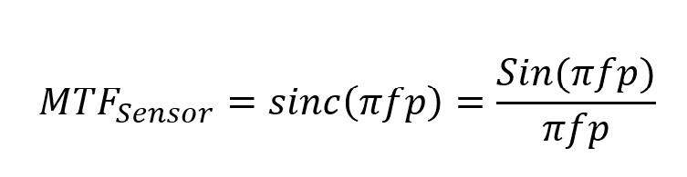
Where f is the spatial frequency (in cycles per mm) and p is the pixel width (which of course is also in mm in the equation).
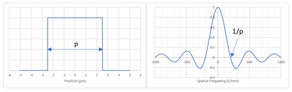
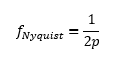
The left plot above shows a RECT function representing a 5µm square pixel. The right plot is the Fourier Transform of the square pixel which is a sinc function. Actually, since the pixel is 2D the sinc function is 2D as well; we are just seeing the cross section. The plot is shown out to 1000 c/mm and the first zero is at 200 c/mm which corresponds to a spatial frequency of 1/pixel width. This plot tells us that broad lines covering many pixels (low spatial frequency) will be resolved with high contrast and that fine lines of 200 c/mm will not be resolved at all. The plot is usually shown with only positive frequencies and y values (MTF) in absolute terms with only positive values. The oscillations in the plot may also be ignored. They are not relevant since they are well above the Nyquist frequency which, in this case, is 100 c/mm. The Nyquist frequency corresponds to 1 wave over 2 pixels and above this frequency aliasing begins to occur in images.
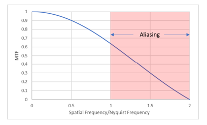
The plot below shows the sinc function out to twice the Nyquist frequency. You will often see this plot in the literature as representative of the MTF of a sensor.
So, why is the sensor MTF given by the Fourier Transform of a pixel shape?
It derives from the fact that the MTF is determined from a convolution of the pixel shape and a series of sine waves across the bandwidth. Mathematically, convolving two functions is the same as multiplying their Fourier Transforms. The Fourier Transform of a range of sine waves is a constant, so the product is simply the Fourier Transform of the RECT function alone.
This may well be mathematically rigorous, but I don’t find it easy to visualize. In the past I have done a pretty simple one-dimensional numerical analysis to visualize a series of pixels receiving a linear sine wave image. Here are some examples.
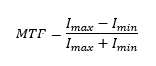
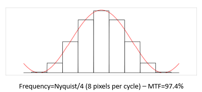
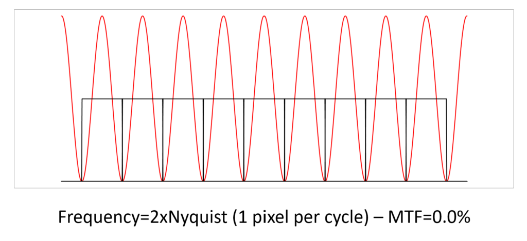
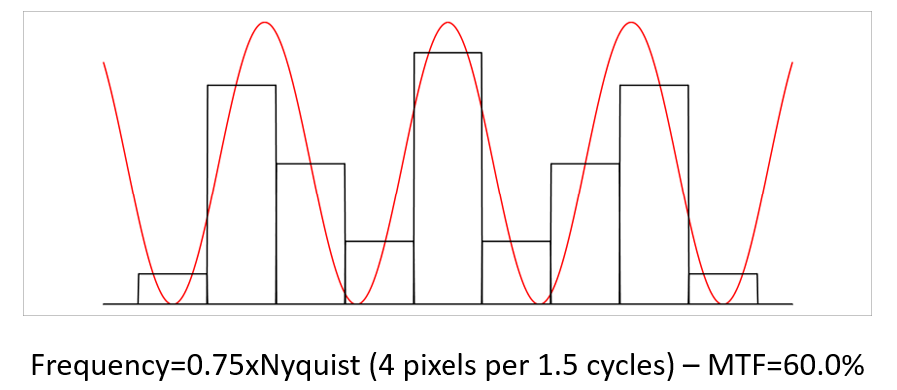
Consider the plots below. The red sine wave represents the illumination pattern, and the black rectangles represent pixels where the height is given by the integration of that part of the sine wave over the pixel width. The sine wave has 100% modulation but because the pixels have a finite size the integration over the pixel width means the sensor always has <100% MTF, as calculated by the usual formula:
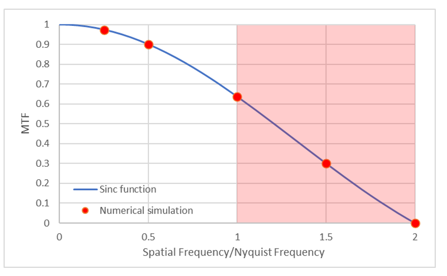
The top plot below represents a low frequency of a quarter of Nyquist frequency and so the pixels with maximum and minimum irradiance have close to 100% and 0% respectively. Numerical simulation tells us that the MTF is 97.4%.
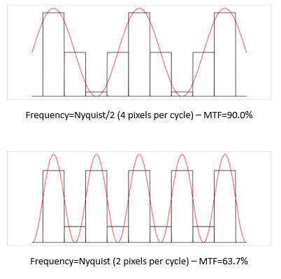
As the illumination pattern frequency increases the max and min pixels depart further from 100% and 0%. At Nyquist/2 the MTF drops to 90% and at Nyquist frequency the MTF is 63.7%.
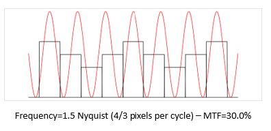
We know that above Nyquist we expect to see aliasing, and this is demonstrated nicely in the plot below. The MTF is 30% but the spatial frequency represented on the sensor is completely wrong.
At twice the Nyquist frequency we have 1 cycle per pixel, and we don’t see any contrast on the sensor.
When we show the numerical simulation results on the MTF plot we see the points fit perfectly.
So, what’s the problem?
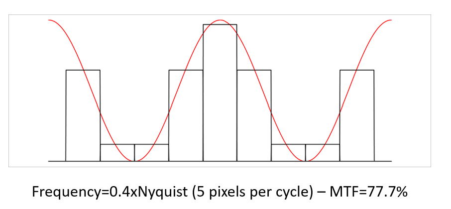
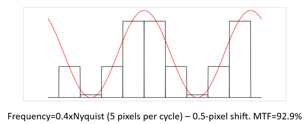
Well, this is only half of the story. The frequencies in the above plots were specially selected to have peaks and valleys of the sine waves precisely centered on a pixel. What happens if they are not? This can be due to a phase shift between the illumination sine wave and the pixels or due to a spatial frequency where 1 wave corresponds to an odd number of pixels, as in the example below.
So where does this fit in the MTF plot?
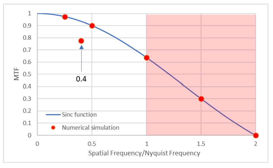
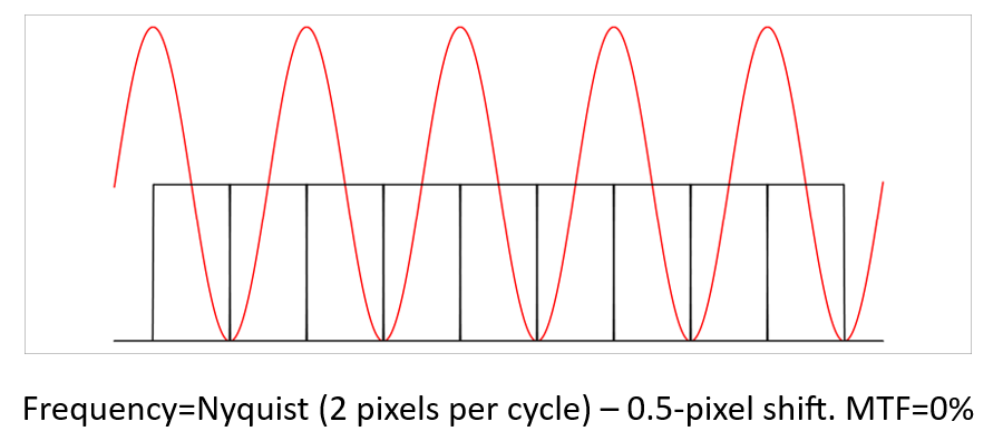
The 0.4xNyquist condition above is definitely not on the sinc function curve (which would be 93.5%). Why is that? Well, the sinc function calculates the MTF based on the pixels that are illuminated with the peaks and valleys of the illumination sine wave. In this example the central pixel coincides with the sine wave peak, but the minima are always at the border of two pixels. If you shift the sine wave phase by half a pixel the minima will then be centered on pixels but now the peak is between pixels (see plot below). In fact, at this frequency condition (1 wave = odd number of pixels) the max and min pixel values never occur in the same image and so the sinc function is wrong at these frequencies.
There are other anomalies. We saw above that at Nyquist the sensor MTF is 63.7% but if we shift the illumination pattern half a pixel, we get zero contrast as shown below. Other phase positions have MTFs between zero and 63.7%.
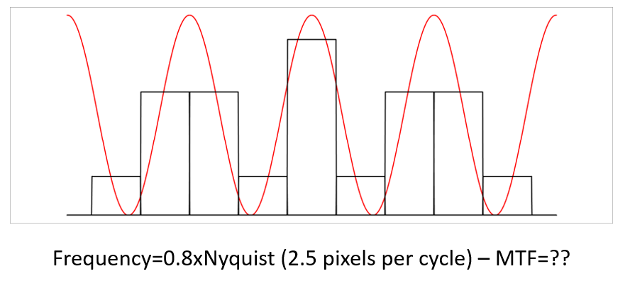
Consider the spatial frequency of 0.8xNyquist in the plot below. All low pixels have the same minima but there are two different pixel maxima. What is the MTF for this frequency?
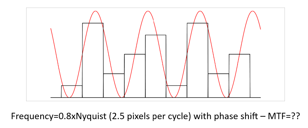
The plot below is the same frequency but with a small phase shift. There are several maxima and minima values.
In this example below (at 0.75xNyquist) we see the center pixel coinciding with the sine wave peak and end pixels coinciding with sine wave valley. Comparing these pixels gives an MTF of 78.4%. This agrees with the sinc function but the max and min pixels don’t occur in the same sine wave so that can’t be correct. If you consider the pixels either side of the center peak as minimum the MTF is 60%. Not so straight forward is it?
The reason for all this confusion is that there are two contributions to the sensor MTF. The first is called the Footprint MTF, the second is the Sampling MTF. The actual sensor MTF is the product of the two. The initial examples with cherry-picked frequencies represented the Footprint MTF.
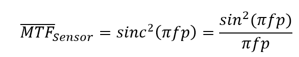
Sampling MTF is often overlooked and accounts for the phase between the pixels and the illumination sine wave. I have seen it not included when a sensor MTF is measured, presumably because the measurement process can include an alignment between the sensor and the illumination pattern. Sampling MTF is also a convolution of the pixel shape and sine wave giving the same sinc function as the Footprint MTF. Hence, the sensor MTF is a sinc-squared function.
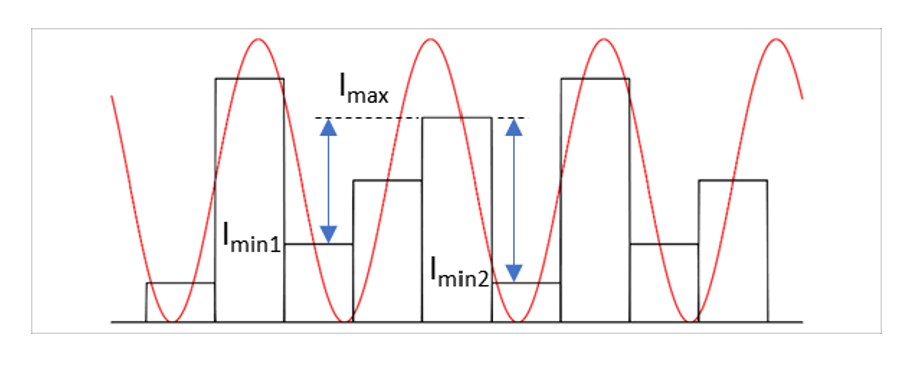
Again, this is not easy to visualize so I did another numerical analysis. In my numerical analysis I took the pixel value of the central sine wave peak as the Imax value and mean of the two pixels at the neighboring minima (Imin1 and Imin2) as the Imin value (shown below). I then stepped the sine wave N times over 1 wave to create a set of N MTF values from which I generate an average for that frequency.
The results of this simulation are shown in the next plot. As you can see the numerical simulation fits perfectly on the sinc2 function.
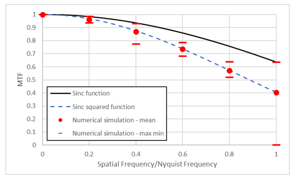
What this all means is that the sensor MTF at any spatial frequency can have a range of values depending on the phase of the illumination sine wave with respect to the pixels. The maximum possible value is given by the sinc function (usually) and the mean MTF is given by the sinc2 function.
If you are told the sensor has an MTF of around 63% at Nyquist frequency it means the Sampling MTF is being ignored.