The Lagrange Invariant Strikes Again!!

Imagine this.  You’ve been asked if you can optimize the design of an illuminator to improve the efficiency, that is, get more light on to a detector.   Increasingly higher power LEDs have been tried but to no avail.  Your immediate reaction is “ah, the Lagrange Invariant strikes again!!” 

Much of the optics world has people using optics in systems in which the primary technology is electronics, sensors, chemistry, or biology etc.  Such clients know plenty of optics but will confess they are not experts and one area they are usually not familiar with is the parameter, étendue. 

Étendue is the two-dimensional cousin of the one-dimensional Lagrange Invariant (and is analogous to the Beam Parameter Product used in Gaussian laser systems).  Each is basically a product of angle and dimension and describe the optical throughput of the system, that is, the limit of how much light you can get from one place to another.  Étendue is French for extent and you may have seen the terms Geometrical Extent or Optical Extent.  Étendue is the parameter commonly used illumination systems.  In any optical system there will be a location of minimum étendue, and that location defines the étendue limit.  

Étendue is defined as:

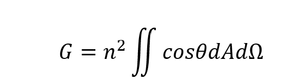
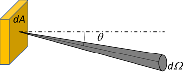
Where n is the refractive index of the medium (usually 1), A is the area, Ω is the solid angle of a beam at an angle θ to the plane of interest, as per the diagram below. 

Most people, however, apply an approximated version of the equation, which is sufficient for most beam angles, as the graph below shows.  

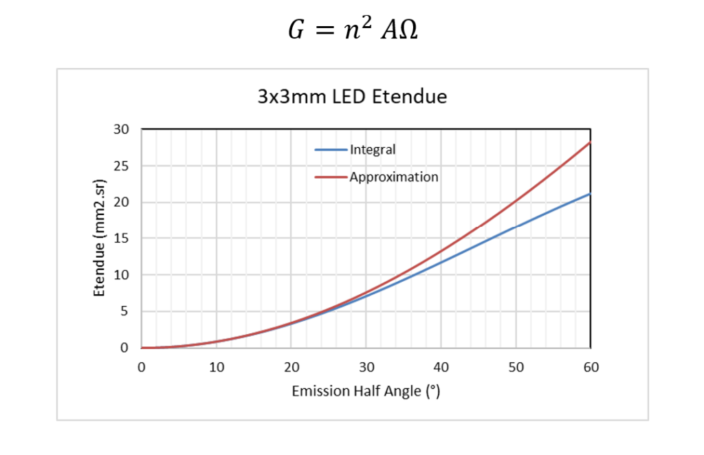
The units of étendue are mm²sr, although some people would say that steradian is not actually a unit (since it’s a ratio) and insist that the unit should be just mm².  There doesn’t seem to be a standard symbol for étendue.  I have seen G used (presumably coming from Geometrical Extent), but also Φ, U, δ, ξ, and ε. Here I use G.

So, how do we apply étendue to a practical example?

Consider you have system where you want to use an LED to illuminate a sample of some sort and then focus the light on to a 1mm square detector.  Let’s say the LED has an emission area of 3x3mm and you are limited to a 0.5NA collection angle at the detector.  The optical layout would be something like this:

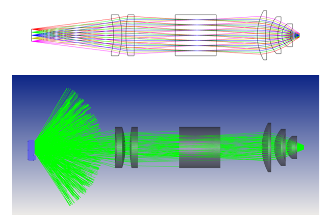
LEDs tend to emit light over 2π steradians. For convenience, let’s assume the emission is +/-60°.  The graph above tells us the étendue is about 21 mm²sr (for that emission angle) but of course most of that light is lost (as the 3D layout shows). 

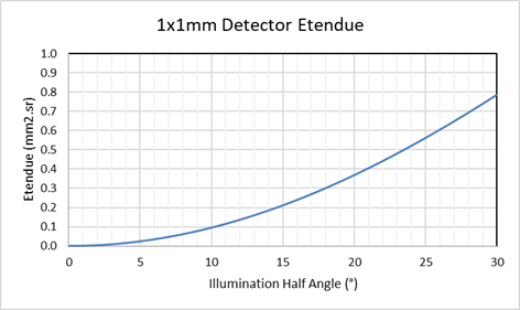
So, how much light do we expect to collect on the detector?  The collection NA is 0.5, which means the collection half angle is 30° and the detector étendue is 0.79 mm²sr (see graph above).  If the emission étendue is 21 mm²sr and the collection étendue is 0.79 mm²sr, that tells us the collection efficiency is going to be about 3.8%. 

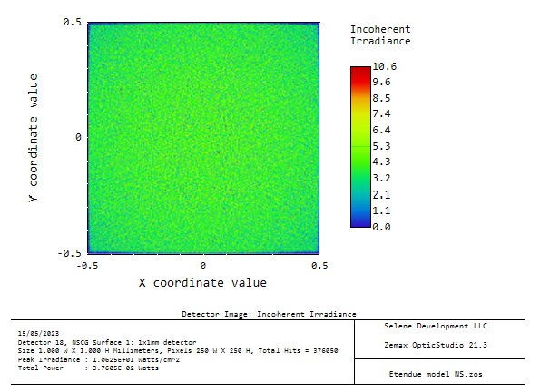
What does an optical simulation tell us about the efficiency?  The simulation result below (with any absorption or reflection losses ignored) shows that for a normalized LED emission of 1W, 37.6mW is received at the detector. That is, 3.76% system efficiency.  Pretty close to the calculation!  A first order étendue estimate would give 3% efficiency. Still not too bad. 

Hence, for this system the detector is the étendue limit of the system and no amount of optical designer magic can squeeze 21 mm²sr into 0.79 mm²sr.  The only levers the designer has available are LED area and the emission angle that the optics should be designed around.  The combination can be a free choice of large area and small angle or vice versa.  There is one caveat to this.  Étendue is a purely geometric optics parameter in which there is an implicit assumption of uniformity (spatial and angular).  If the emission half angle is 60° but strongly peaking at low angles, it would be more efficient to design the optics for a large area and small angle.  Conversely, if the source has a central hot spot (like some thermal sources) it would be better to design for a small area and large angle.

The calculation of the system étendue limit is the starting point of an illuminator design and points the designer in the right direction to complete the task. 

One last point, étendue has its roots in thermodynamics and entropy*.  As with entropy, it is not possible to reduce étendue, but it is possible to increase it.  For example, consider a collimated laser beam.  This is well known to be a very low etendue source.  With an appropriate lens such a beam can be focused to a small spot.  But if you direct that beam through a diffuser, you break the wavefront and create a new set of source points.  This is analogous to increasing disorder on the system. From this point in the optical system the étendue is calculated from the spot size on the diffuser and the scatter angle, and it will not be possible to focus the beam to anywhere near the same spot size as without the diffuser.

We’ll return to étendue at a later date to cover more complex examples like beamsplitters and fly’s eye homogenisers.

*Markvart, T. “The thermodynamics of optical etendue”, J. Opt. A: Pure Appl. Opt. 10 (2008) 015008